Mixture PK-YOLO

Brain tumor detection using YOLO-based model

This project is built based on the paper .

Abstract

• MRI slices
  • Axial, coronal, and sagittal imaging views
• PK-YOLO
  • Detect brain tumors from 2D multiplanar MRI slices
  • The backbone is pretrained only in axial views
  • Backbone extracts same axial-biased features for all plane (axial, coronal, and sagittal)

Figure 1. Three planes of MRI brain scans. The brain MRI scans with a 3D structure are cut on axial (green), the coronal (blue), and the sagittal plane (red).

• PK-YOLO uses SparK RepViT as main backbone
  • SparK pretraining strengthens feature extraction, especially axial
• Input: 640x640 MRI slices from different planes such as Axial, Coronal and Sagittal
• Auxiliary CBNet acts as an extra gradient branch that improves feature quality
• Final detection is performed by YOLOv9
• Achieve the highest performance among DETR and YOLO based in the original study

Figure 2. Model architecture of PK-YOLO. By using SparK RepViT as a backbone, the model achieved state-of-the-art performance.

Limitations of the Previous Work

• Pretraining on a single plane data
  • Axial-biased features
  • Same features are applied to other planes
• Large performance gap
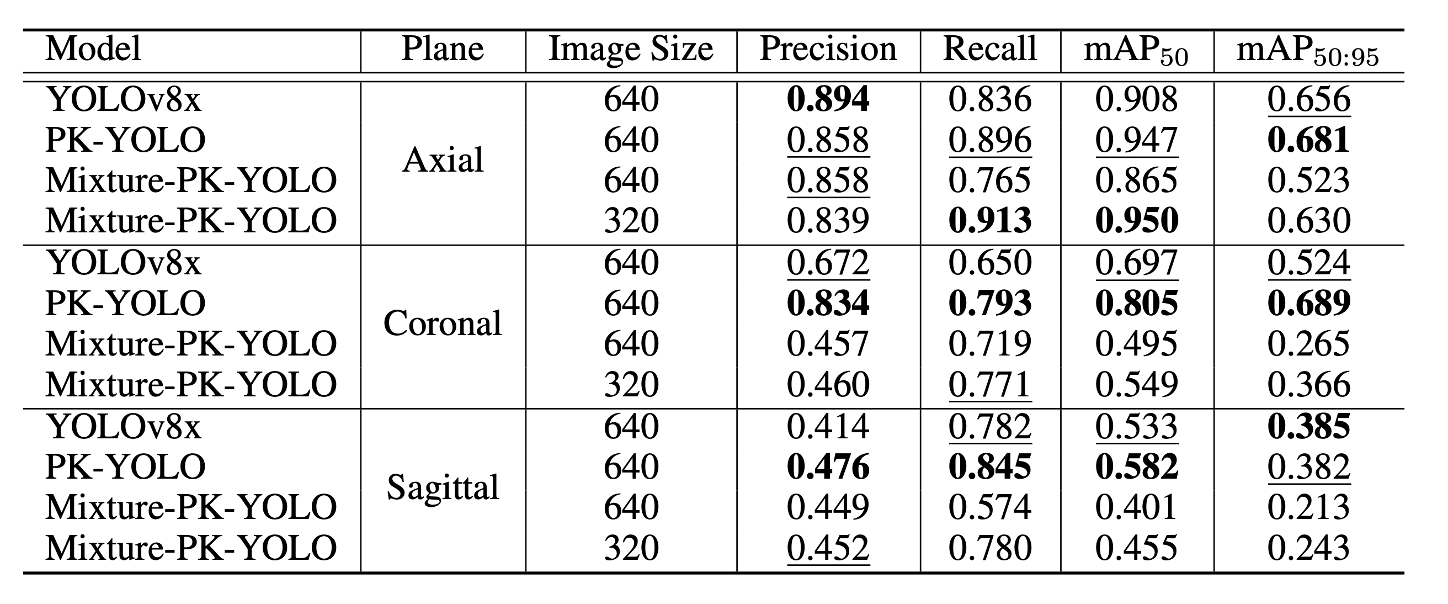
  • Axial \(mAP_{50} \rightarrow 0.947\)
  • Coronal \(mAP_{50} \rightarrow 0.805\)
  • Sagittal \(mAP_{50} \rightarrow 0.582\)

Table 1. PK-YOLO’s performance comparison across different plane datasets.

Related Work

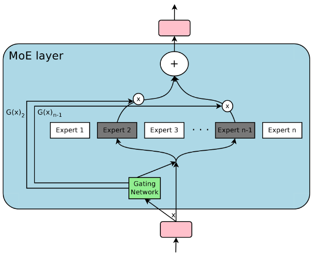
Mixture-of-Experts (MoE)

MoE combines multiple specialized models using a gating layer.

• Each model acts as an expert
  • Gating layer to combine outputs into one
• Advantages
  • Computational efficiency
  • Scalability

Figure 3. A Mixture of Experts (MoE) layer embedded within a recurrent language model.

LION

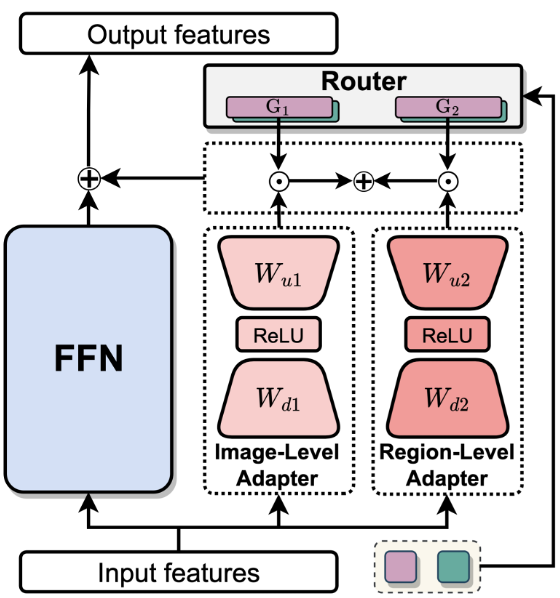
LION uses a router module to balance two types of knowledge.

• Router adjusts the ratio between image-level and region-level knowledge
• Demonstrates how a router weighs two features.

Figure 4. Router module for MLLM (namely LION) to control image-level and region-level knowledge.

For more information, refer to this paper review post.

Method

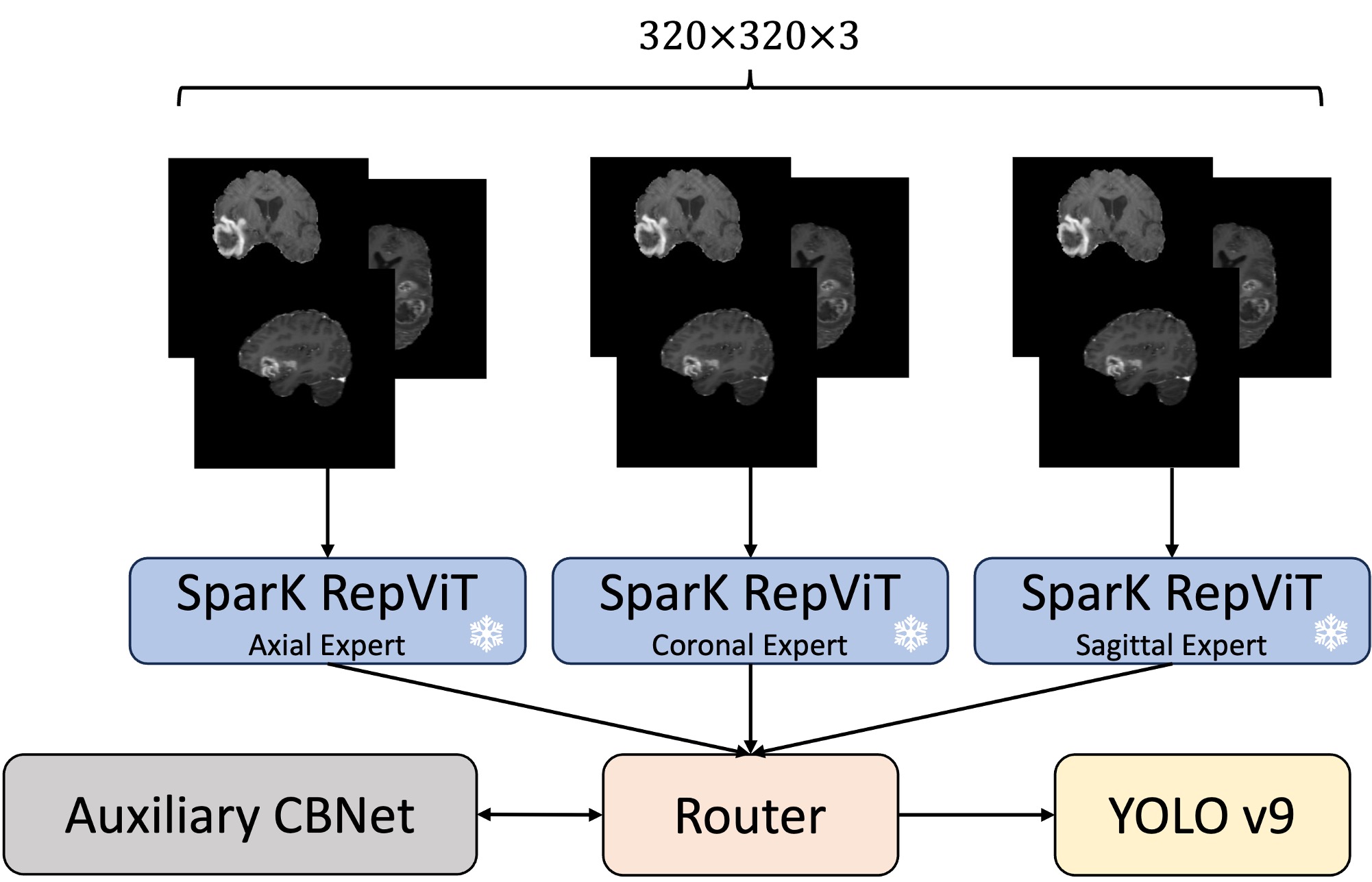
Building on the limitations and insights from related work, the solution to the single backbone architecture seems straightforward. The figure here provides a direct one-to-one comparison between the original PK-YOLO model and our proposed Mixture PK-YOLO model. The main difference between these two architectures is that our model uses three separate backbones, one for each plane, instead of relying on a single pretrained backbone. Additionally, we introduce a router module right after the backbone outputs to effectively combine the plane-specific features.

Figure 5. Comparison of original PK-YOLO and proposed Mixture PK-YOLO model. Instead of having a single pretrained backbone model, Mixture PK-YOLO employs three pretrained and frozen backbones per plane, and uses router module to combine the three outputs into one unified representation.

SparK Pretraining

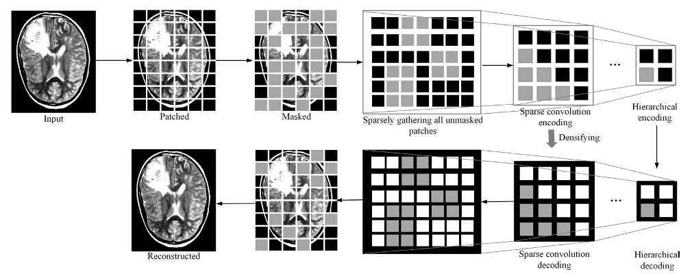
The pretraining process is done using the SparK method. We first start with an MRI slice as an input, which then is divided into patches. And these patches are masked out randomly, leaving unmasked and masked patches. The key idea of SparK method is the sparse convolutions. Instead of processing all patches, sparse convolution only computes on the unmasked patches and completely skips the masked patches.

After the sparse convolutions, unmasked patches are fed into an encoder, followed by a densifying step. The final output is a reconstructed image where the model has learned to infer the masked patches.

Through this SparK pretraining process, the backbone model is equipped with general knowledge of brain tumor image, then used in PK-YOLO architecture for tumor detection.

Figure 6. The process of SparK pretraining for backbone model inside the PK-YOLO.

Model Architecture

• Employs three pretrained backbone models
• Treats each pretrained backbone as an expert in each plane
• Freeze all three backbones
• Router module fuse three outputs from the backbones

Figure 7. Mixture PK-YOLO employs three backbones treating each backbone as an expert to its corresponding plane data. Then a router module integrates the outputs from the backbones into one, then pass it to YOLO model.

Router Module

\[\begin{align*} \tilde{F}_k^{(n)} = AAP(F_k^{(n)}(X)) \in \mathbb{R}^{C_n}, \end{align*}\]

where \(AAP(\cdot)\) is adaptive average pooling layer. Then, the reduced feature maps are given to the score function thtat maps,

\[\begin{align*} & z_k^{(n)} = g_n(\tilde{F}_k^{(n)}(X)) \in \mathbb{R} \\ & \rightarrow \mathbb{z}^{(n)} = [z^{(n)}_1, z^{(n)}_2, z^{(n)}_3 ] \in \mathbb{R}^3. \end{align*}\]

In this work, the score function \(g_n(\cdot)\) is replaced with two-layered simple linear layers with ReLU layer inplaced in between.

Then, the weights are measured for each scores of backbone models’ outputs as such,

\[\begin{align*} w^{(n)}_k = \frac{\exp{(z^{(n)}_k)}}{\sum_{i=1}^{3} \exp{((z^{(n)}_i))}}. \end{align*}\]

The weight \(w^{(n)}_k\) decides which plane to give a higher importance than the other plane information. Given the weights, the router module controls the importance of each backbone’s output as follows,

\[\begin{align*} Z^{(n)} = \sum_{i=1}^{3} w^{(n)}_i \cdot F^{(n)}_i(X). \end{align*}\]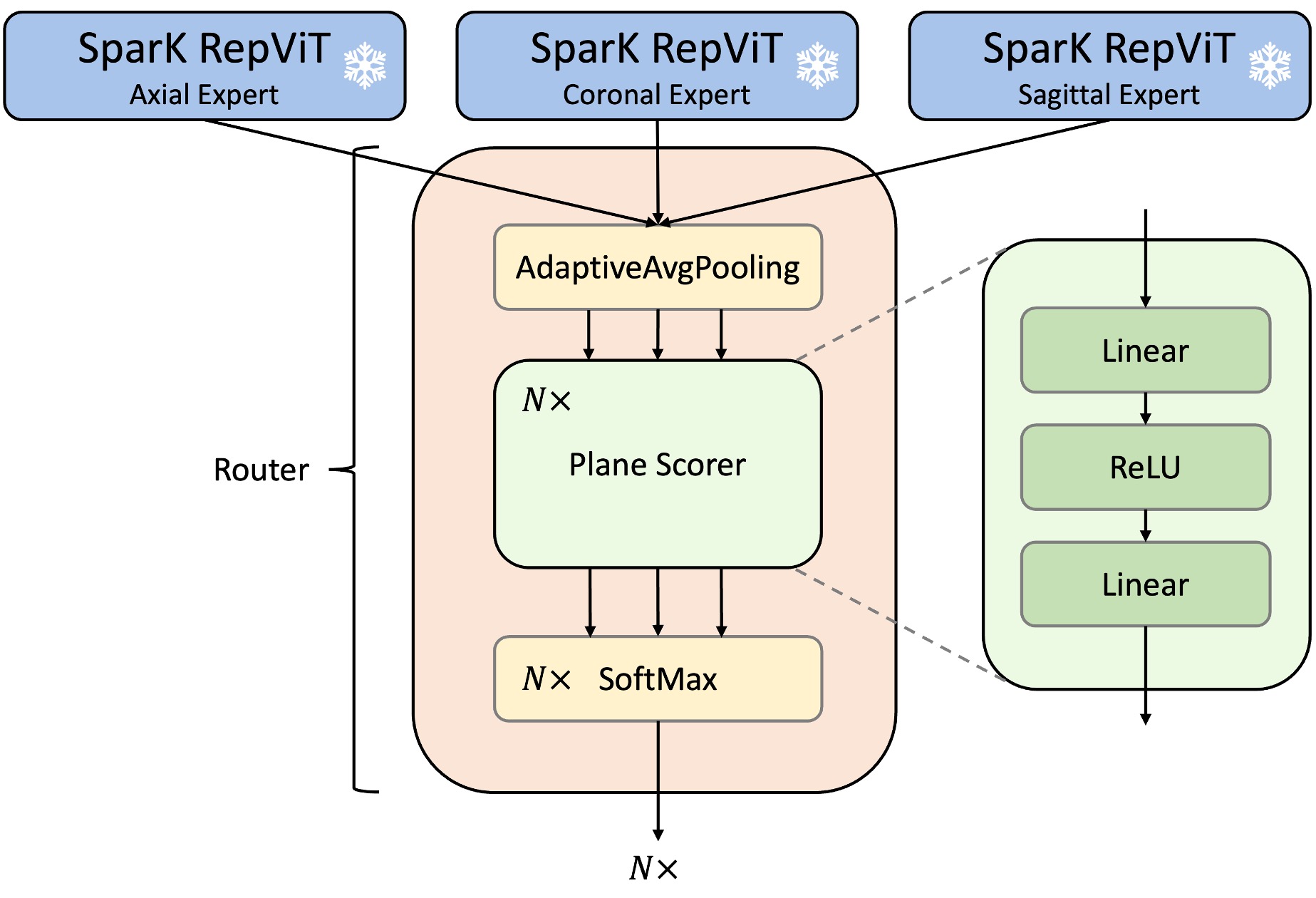

Figure 8. Router module from Mixture PK-YOLO to control the importance of plane-specific information.

Experiments

Fitness Score

\[F = 0.1 P + 0.1 R + 0.3 AP_{50} + 0.5 AP_{50:95}\]

The above uses precision, ** recall, **average precision, and Intersection-over-Union (IoU) metric to evaluate the model performance.

Training Losses

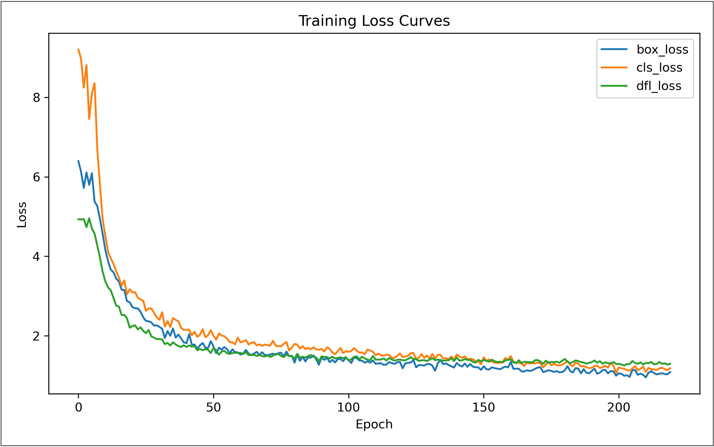
• Box loss: evaluates how accurately the predicted bounding boxes match the ground truth using an IoU-based measure \(\rightarrow\) penalizing poor localization.
• Objectness loss: supervises the model’s confidence in distinguishing object regions from background regions \(\rightarrow\) helping reduce both false positives and false negatives.
• Classification loss: measures how well the model assigns the correct class labels to detected objects \(\rightarrow\) ensuring accurate category discrimination.

Learning Curves

Figure 9. Training result of Mixture PK-YOLO for 300 epochs. Blue (box_loss) represents loss for bounding box, orange (cls_loss) represents classification loss, and green (dfl_loss) represents objectness loss.

Performance Comparison

Table 3. Comparison of model performance across planes. PK-YOLO remains to achieve state-of-the-art performance, and proposed Mixture PK-YOLO achieves reasonable performance, while showing higher Recall and mAP 50 metrics on axial plane.

Ablation Study of Frozen Backbones

Table 4. Ablation study on freezing backbones. Bold numbers show higher performance. Not only does freezing the backbones reduce the amount of training parameters but also increases the overall model performance.

Analysis of the Result

• Effectiveness of Router Module
  • Higher weight ratio to the plane that was given
  • Lower weight ratio to the other planes, instead of 0
  • E.g. given a coronal brain tumor image,
    • The output should be something like \(Z = 0.2 F_{axi}(X) + 0.65 F_{cor}(X) 0.15 F_{sag}(X)\).
  • Further studies on evaluating the router module are required
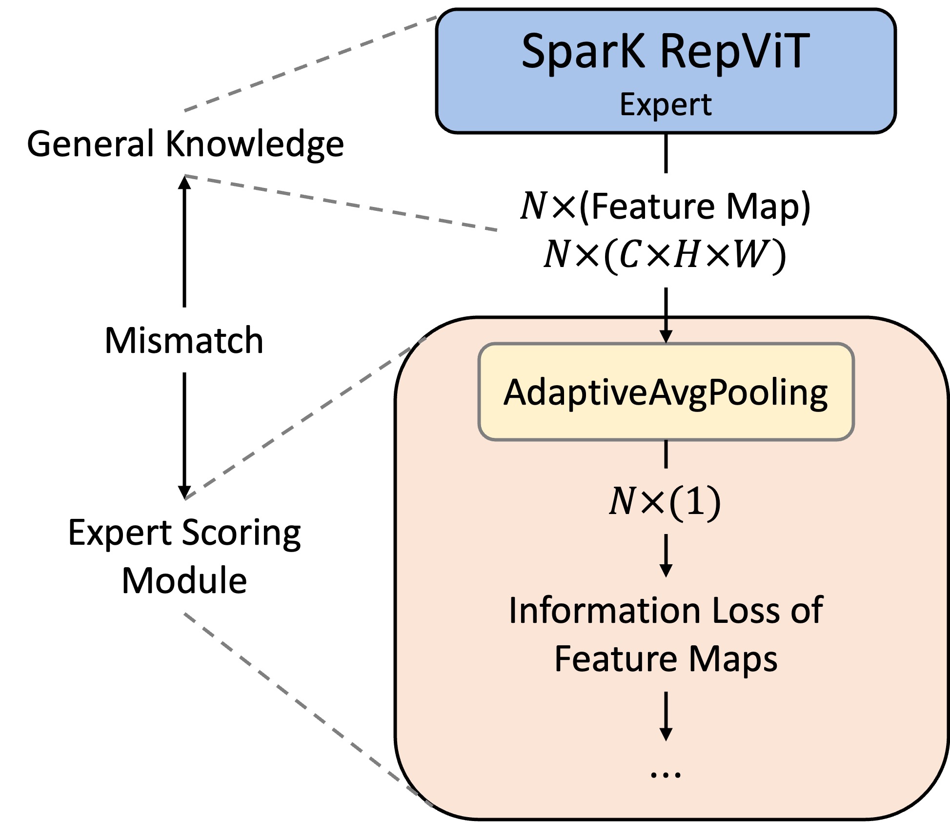
• Discrepancy in the connection
  • Backbone outputs general knowledge of plane-specific brain tumor images
  • Router module scores the importance of the information
  • Average Pooling layer causes severe feature information loss

Figure 10. Detailed look of the connection between a backbone and the router module.

Conclusion

• Introduced three-backbone architecture
  • Each was pretrained and specialized for the axial, coronal, and sagittal planes
• Employed a router module to fuse plane-specific features from the backbones
• Could not reach the state-of-the-art performance of PK-YOLO
  • Demonstrated stronger performance in certain cases (i.e., axial plane)
• Achieved a 49.2% reduction in trainable parameters 
  • Training overhead was significantly reduced