Dynaformer, A Deep Learning Model for Ageing-aware Battery Discharge Prediction
Transformer-based Battery EoD Prediction Model
The review is done with the following paper:
Luca Biggio, Tommaso Bendinelli, Cheta Kulkarni, and Olga Fink. “Dynaformer: A Deep Learning Model for Ageing-aware Battery Discharge Prediction,” Applied Energy, 2023.
Table of Contents
Abstract
The main purpose of the paper is to propose a novel deep learning architecture which can be applied to batteries, namely Dynaformer. The model, Dynaformer, is a Transformer-based [2] model and outputs an EoD (end of discharge) prediction, given some context current and voltage curves.
Dynaformer is able to infer the ageing state from a limited samples and predict the full voltage discharge curve, EoD, simultaneously.
Background
Battery
The following Figure 1. represents how batteries’ voltage curves look like based on the given input current profiles. When given constant current, it forms a continuous curve as the graph on the far left. On the other hand, when given some variable current profiles with multiple transitions, the graphs differ from the other corresponding to the altering current.

Figure 1. Varying voltage curves corresponding to altering current profiles [1]
There are two main categories of solving EoD prediction and ageing inference: model-based method and data-driven method. The first method, model-based method, mainly focuses on representation of battery’s physical internal mechanism. By constructing an ideal model of the battery, it has a good performance. However, due to it’s complex representation of the model, it is computationally expensive and is not an easy work to design the model precisely.
The second method, data-driven method, is to predict EoD and ageing inference using a huge amount of battery data. It is easier to model the system compared to the model-based method since it requires minimum prior knowledge on the battery’s discharge and degradation processes. Nevertheless, it also has some disadvantages. It requires large labeled training dataset and it is inefficient to train with such long time series data.
Transformer
It is essential to understand how Transformer [2] works in order to understand the Dynaformer. Let’s consider the following sentence.
The dog is playing and she likes playing with me.
We know that she is indicating the dog, not me. Transformer is all about understanding the context and the hidden meaning behind the given data.


Figure 2. Transformer model architecture [2]. (Left) Positional embedding (Centre) Encoder (Right) Decoder
Transformer is consists of three major parts: positional embedding, encoder and decoder. The above Figure 2. represents the mentioned three parts.
Positional embedding is to transfer the given data into numerical vectors. By doing so, positional information can be embedded within the vectors.
Encoder’s job is to obtain query, key and value – \((Q, K, V)\) – given some positional embedding. The query is a vector which contains given specific data such as a word itself when a sentence is given. The key is a value which can specify the query. And lastly, the value represents the query’s hidden meaning. It can contain context or positional information. Here, self-attention comes in. Simply saying, self-attention cells find the correlations among the data by using \((Q, K, V)\).
Decoder’s job is very similiar with the encoder but it differs with the main purpose. While the encoder’s main purpose is to find the correlations among input data, the decoder’s main purpose is to find the correlations between the input data and ouput data.
To simplify, let’s bring the classic translation example. Say I want to translate some English sentences into Korean sentences. Then the input of the encoder is the English sentences and the input of the decoder is the the Korean sentences, in other words, data that we target. So the encoder mainly interprets and finds the meaning, hidden information, and correlations from the English sentences, and the decoder focuses on finding the correlations between the English sentences and the Korean sentences, when training.
Back to the point, the decoder also obtains query, key, and value. However, in the decoder, key and value from the encoder and query from decoder will only be used. By using \((K, V)\) from the encoder and \((Q)\) from the decoder, the decoder is able to apply self-attention mechanism to find the correlations between the data we want to interpret and the data we aims.
Model Architecture
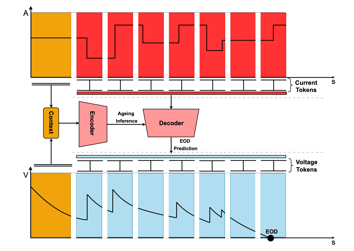
Figure 3. Representation of the components of Dynaformer [1]
The proposed Dynaformer is basically the same with the Transformer model but with the difference of the data type. Since the paper is to predict EoD, input data types are current and voltage curves. Note that the inputs of the encoder are current and voltage curves and the inputs of the decoder are the rest of the current curves and the output of the encoder, then eventually outputs full discharge voltage curves.

Figure 4. Dynaformer - model architecture [1]
Figure 3. and Figure 4. are the same model architecture, but for the sake of easy understanding of the Dynaformer using the Transformer-style architecture representation, Figure 3. can be redrawn as Figure 4.. The following figures specify each part from the Dynaformer.


Figure 4-1, 4-2, 4-3. Dynaformer - detailed model architecture [1]. (Left) Positional embedding (Centre) Encoder (Right) Decoder
Embedding

Figure 5. Dynaformer - (Context) Embedding [1]
Here, Dynaformer gets information regarding the battery’s profiles, which are current profile (curve) and voltage profile (curve). While (positional) embedding, nothing special happens but reshapes the data into \((Q, K, V)\) including positional, context information. The \(Q\) represents current and voltage curves, the \(K\) serves as a specifier to find the \(Q\), and the \(V\) contains positional information such as time for the matching \(Q\).
Encoder

Figure 6. Dynaformer - Encoder
The encoder’s inputs are \((Q, K, V)\) from the embedding. Here, it’s main role is to find the correlations between the input current, voltage, and time which will eventually extracts degradation information. In order to find such information, multi-head self-attention cells are used. For further information regarding self-attention mechanism, please see [2].
Decoder

Figure 7. Dynaformer - Decoder [1]
The decoder predicts EoD as a final ouput, given the ageing inference from the encoder’s ouput and the rest of the current curves which are from the decoder’s input. Using the ageing inference, \((K, V)\), and the rest of the current curves, \(Q\), the Dynaformer is now able to predict the voltage curves corresponding to the current curves from the input of the decoder exploiting the ageing inference information from the encoder.
Solutions for The Limitations
Just like I’ve mentioned from the Background - Battery section, there are two main limitations when using data-driven method for predicting EoD and ageing inference: requires large labeled dataset and requires long time series dataset which is inefficient for training.
The proposed Dynaformer solves the problems originally had when using data-driven method.
First, the Dynaformer mitigated the problem of lack of dataset for training by using the following: [3] and [4]. [3] is a NASA Prognostics Model library which helps creating a simulated training dataset. The paper experiments the model by changing two degradation parameters, \(q_{max}\) and \(R_0\), to observe the performance change when the parameters changed. Also [4] is a NASA real-world Dataset for batteries and is used as a input for the simulator, [3].
However, there may be a simulation-to-real gap (sim2real gap) since the training dataset is a simulation-based data. To mitigate such concern, the paper applied transfer learning. As [5] suggests, training the model with simulated data then using a limited amount of real data to adapt the model can reduce the model’s bias towards simulated data.
Second, the Dynaformer gets the tokenized input. In other words, instead of feeding a full length of the curves, the Dynaformer only accepts a small sized curves in sequence. Please see Figure 3. for better understanding of the concept of token. Training the model with long time series data is in fact inefficient. However, using the technique from [6] solves such problem.
Results
Experimental Setup
Two metrics will be used to evaluate the performance of the model namely RMSE (Root Mean Squared Error) and RTE (Relative Temporal Error). You might be familiar with RMSE but not RTE. The RTE is a error evaluating metric, which the paper proposed, inspecting the maximum error when given a longer or shorter input profile. It measures how the model behaves when the input size is longer or shorter than usual measuring the maximum error, so the authors call the RTE metric a worst case performance measurement.
The following is the algorithm for measuring the RTE metric [1].

Performance Evaluation
Please see the following Table 1. for the evaluation. As described from Results - Experimental Setup section, two metrics, RMSE and RTE, will be used to evaluate the performance of the model. For the comparison, LSTM model and FNN model will be used for simulated data. Note that since FNN model can not handle variable-sized input, only the LSTM model will be compared. And for the final evaluation, real data will be used to see the performance of the Dynaformer model using two metrics.
| LSTM | FNN | ||||
| Metrics | |||||
| RMSE | RTE | ||||
| Simulated data | |||||
| Constant current | O | O | X | O | |
| Variable current | O | X | O | O | |
| Real data | X | X | O | O | |
Table 1. Performance evaluation
Simluated Constant Current Profiles

Figure 8. Results on constant load profiles [1]. (Left) Interpolation performance. Altering degradation values in the same range to the training set. (Right) Extrapolation performance. Altering degradation values in the different range to the training set. Dynaformer with a asterisk (*) denotes the model trained with variable profiles.

Figure 9. Generalization performance analysis with respect to degradation parameters. [1]. The grey-coloured area represents the interpolation region. Fixed current of 1A (left) and 2A (right).
Simluated Variable Current Profiles

Figure 10. Results on variable load profiles using Dynaformer [1]. (Left) Interpolation performance. Altering degradation values in the same range to the training set. (Right) Extrapolation performance. Altering degradation values in the different range to the training set.

Figure 11. Illustration of the Dynaformer's prediction with respect to the numbers of transitions of current [1].
Implicit Ageing Inference

Figure 12. Implicit parameters inference [1]. With the use of encoder's output information, two principal components, one can infer the corresponding degradation parameters by inspecting the following areas. (Left) Shows high correlations between q_max and the second principal component. (Right) Shows high correlations between R_0 and the first principal component.
Real data

Figure 13. Adaption to real data via fine-tuning [1]. Close the gap between simulation-to-real gap by showing small fraction of real data to the pre-trained model. (a) Sim2Real gap (b) Performance before / after fine-tuning (c) MSE distribution before / after fine-tuning (d) RTE measurements according to the number of real data used to train
Note. Optimal performance can already be obtained with smaller training sizes.
Conclusion
- Dynaformer (Transformer-based EoD prediction model)
- Proposed three possible extension works:
- Apply the proposed methodology to alternative simulators
- Exploit the characteristic that the model represents differentialbe simulator
- Gradient-based methods can be used to specify when the voltage trajectory leads to discharge
- Apply the Dynaformer to learning very different system dynamics
Reference
[1] Luca Biggio, Tommaso Bendinelli, Cheta Kulkarni, and Olga Fink. “Dynaformer: A Deep Learning Model for Ageing-aware Battery Discharge Prediction,” Applied Energy 2023.
[2] Ashish Vaswani, Noam Shazeer, Niki Parmar, Jakob Uszkoreit, Llion Jones, Aidan N. Gomez, Lukasz Kaiser, and Illia Polosukhin. “Attention is All you Need,” Advances in Neural Information Processing Systems 30 (NIPS 2017), 2017.
[3] Chris Teubert, Katelyn Jarvis, Matteo Corbetta, Chetan Kulkarni, Portia Banerjee, Jason Watkins, and Matthew Daigle, “ProgPy Python Prognostics Packages,” v1.6, Oct 2023. URL https://nasa.github.io/progpy/index.html
[4] B. Saha and K. Goebel (2007). “Battery Data Set”, NASA Prognostics Data Repository, NASA Ames Research Center, Moffett Field, CA.
[5] Sun, Chi, Xipeng Qiu, Yige Xu, and Xuanjing Huang. “How to fine-tune bert for text classification?.” In Chinese Computational Linguistics: 18th China National Conference, CCL 2019, Kunming, China, October 18–20, 2019, Proceedings 18, pp. 194-206. Springer International Publishing, 2019.
[6] Alexey Dosovitskiy, Lucas Beyer, Alexander Kolesnikov, Dirk Weissenborn, Xiaohua Zhai, Thomas Unterthiner, Mostafa Dehghani et al. “An image is worth 16x16 words: Transformers for image recognition at scale.” arXiv preprint arXiv:2010.11929 (2020).
References
2022
-
 Dynaformer: A Deep Learning Model for Ageing-aware Battery Discharge Prediction2022
